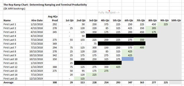
Kellblog covers topics related to starting, leading, and scaling enterprise software startups including strategy, marketing, positioning, messaging, management, go-to-market, SaaS metrics, and venture capital financing.
In prior posts I have discussed how to make a proper sales bookings productivity model and how to use the concept of ramped rep equivalents (RREs) in sales analytics and modeling. When it comes to setting drivers for both, corporate leaders tend to lean towards benchmarks and industry norms for the values. For example, two such common norms are:
Setting steady-state (or terminal) productivity at $1,200K of new ARR per rep in enterprise SaaS businesses
Using a {0%, 25%, 50%, 100%} productivity ramp for new salesreps in their {1st, 2nd, 3rd, 4th} quarters with the company (and 100% thereafter)
In this post, I’ll discuss how you can determine if either of those assumptions are reasonable at your company, given its history.
To do so, I’m introducing one of my favorite charts, the Rep Ramp Chart. Unlike most sales analytics, which align sales along fiscal quarters, this chart aligns sales relative to a rep’s tenure with the company.
You start by listing every rep your company has ever hired [1] in order by hire date. You then record their sales productivity (typically measured in new ARR bookings [2]) for their series of quarters with the company [3], up to and including their current-quarter forecast (which you shade in green). Reps who leave the company are shaded black. Reps who get promoted out of quota-carrying roles (e.g., sales management) are shaded blue. Future periods are shaded grey. Add a 4+ quarter average productivity column for each row, and average each of the figures in the columns [4].
Here’s what you get:
Despite having only a relatively small amount of data [5], we can still interpret this a little.
The relative absence of black lines means we’re pretty good at sales hiring. I’ve seen real charts with 5 black lines in a row, usually down to a single bad management hire.
The absence of black lines that “start late” — for example {0, 25, 75, 25, 55, black} — is also good. Our reps are either “failing fast” or succeeding, but things are not dragging on forever when they’re not working.
Our average 4Q+ productivity is $308K per quarter, almost exactly $1,200K per year so it does seem valid to use that figure in our modeling.
Entering $300K as target productivity then shows the empirical rep ramp as a percent of steady-state productivity, exactly how sales leaders think of it. In this case, we see a {10%, 38%, 76%, 85%, 98%} empirical ramp across the first five quarters. If our bookings model assumed {0%, 25%, 50%, 100%, 100%}, you’d say our model is somewhat pessimistic in the first three quarters, a little optimistic in the 4th, and pretty much on-target (a tiny bit optimistic) in the 5th. If we had more data, we might adjust it a bit based on that.
I love this chart because it presents unadulterated history and lets you examine the validity of two hugely important drivers in your sales bookings capacity model — drivers, by the way, that are often completely unquestioned [6]. For that reason, I encourage everyone to make this a standard slide in your Sales ops review (aka, QBR) template. Note that since different types of rep ramp differently and hit different steady-state productivity levels, you should create one rep ramp per major type of rep in your company. For example, corporate (or inside) sales reps will typically ramp more quickly to lower productivity levels than field reps who will ramp more slowly to higher productivity. Channels reps will ramp differently from direct reps. International reps may need their own chart as well.
[1] Sales management may want to omit those no longer with the company, but that also omits their data, and might omit important patterns of hiring failure, so don’t omit anyone. You can always exclude certain rows from the analysis without removing them from the chart (i.e., hiding them).
[2] New ARR bookings typically includes new ARR to both new and existing customers.
[3] You’ll need as many columns to do this as your longest tenured rep has been with the company, so it can get wide. Let it. There’s data in there.
[4] Ensuring empty cells are not confused with cells whose value is zero. Excel ignores empty cells in calculating averages but will average your 0’s in when you probably don’t want them.
[5] In order to keep it easily and quickly grasped
Enterprise SaaS and retailers have more in common than you might think.
Let’s think about retailers for a minute. Retailers drive growth in two ways:
They open new stores
They increase sales at existing stores
Opening new stores is great, but it’s an expensive way to drive new sales and requires a lot of up-front investment. It’s also risky because, despite having a small army of MBAs working to determine the right locations, sometimes new locations just don’t work out. Blending the results of these two different activities can blur what’s really happening. For example, consider this company:
Things look reasonable overall, the company is growing at 17%. But when you dig deeper you see that virtually all of the growth is coming from new stores. Revenue from existing stores is virtually flat at 2%.
It’s for this reason that retailers routinely publish same-store sales in their financial results. So you can see not only overall, blended growth but also understand how much of that growth is coming from new store openings vs. increasing sales at existing stores.
Now, let’s think about enterprise software.
Enterprise software vendors drive growth in two ways:
They hire new salesreps
They increase productivity of existing salesreps
Hiring new salesreps is great, but it’s an expensive way to drive new sales and requires a lot of up-front investment. It’s also risky because, despite having a small army of MBAs working to determine the right territories, hiring profiles and interviewing process, sometimes new salesreps just don’t work out. Blending the results of these two different activities can blur what’s really happening. For example, consider this company:
If you’re feeling a certain déjà vu, you’re right. I simply copy-and-pasted the text, substituting “enterprise software vendor” for “retailer” and “salesrep” for “store.” It’s exactly the same concept.
The problem is that we, as an industry, have basically no metric that addresses it.
Revenue, bookings, and billings growth are all blended metrics that mix results from existing and new salespeople [1]
Retention and expansion rates are about cohorts, but cohorts of customers, not cohorts of salespeople [2]
Sales productivity is typically measured as ARR/salesrep which blends new and existing salesreps [3]
Sales per ramped rep, measured as ARR/ramped-rep, starts to get close, but it’s not cohort-based, few companies measure it, and those that do often calculate it wrong [4]
So what we need is a cohort-based metric that compares the productivity of reps here today with those here a year ago [5]. Unlike retail, where stores don’t really ramp [6], we need to consider ramping in defining the cohort, and thus define the year-ago cohort to include only fully-ramped reps [6].
So here’s how I define same-rep sales: sales from reps who were fully ramped a year ago and still here.
Here’s an example of presenting it:
The above table shows same-rep sales via an example where overall sales growth is good at 48%, driven by a 17% increase in same-rep sales and an 89% increase in new-rep sales. Note that enterprise software is a business largely built on the back of sales force expansion so — absent an acquisition or new product launch to put something new in sale’s proverbial bag — I view a 17% increase in same-rep sales as pretty good.
Let’s conclude by sharing a table of sales productivity metrics discussed in this post that I think provides a nice view of sales productivity as related to hiring and ramping.
The spreadsheet I used for this post is available for download, here.
# # #
Notes
[1] Billings is a public company SaaS metric and typically a proxy for bookings.
[3] Public companies never release this but most public and private companies track it.
[4] By taking overall new ARR (i.e., from all reps) and dividing it by the number of ramped reps, thus blending contribution from both new and existing reps in the numerator. Plus, these are usually calculated on a snapshot (not a cohort) basis.
[5] This is not survivor-biased in my mind because I am trying to get a productivity metric. By analogy, I believe stores that closed in the interim are not included in same-store sales calculations.
[6] Or to the extent they do, it takes weeks or months, not quarters. Thus you can simply include all stores open in the year-ago cohort, even if they just opened.
[6] I am trying to avoid seeing an increase in same-rep sales due to ramping — e.g., someone who just started in the year-ago cohort will have year sales, but should increase to full productivity simply by virtue of ramping.
I’ve seen numerous startups try numerous ways to calculate their sales capacity. Most are too back-of-the-envelope and too top-down for my taste. Such models are, in my humble opinion, dangerous because the combination of relatively small errors in ramping, sales productivity, and sales turnover (with associated ramp resets) can result in a relatively big mistake in setting an operating plan. Building off quota, instead of productivity, is another mistake for many reasons [1].
Thus, to me, everything needs to begin with a sales productivity model that is Einsteinian in the sense that it is as simple as possible but no simpler.
What does such a model need to take into account?
Sales productivity, measured in ARR/rep, and at steady state (i.e., after a rep is fully ramped). This is not quota (what you ask them to sell), this is productivity (what you actually expect them to sell) and it should be based on historical reality, with perhaps incremental, well justified, annual improvement.
Rep hiring plans, measured by new hires per quarter, which should be realistic in terms of your ability to recruit and close new reps.
Rep ramping, typically a vector that has percentage of steady-state productivity in the rep’s first, second, third, and fourth quarters [2]. This should be based in historical data as well.
Rep turnover, the annual rate at which sales reps leave the company for either voluntary or involuntary reasons.
Judgment, the model should have the built-in ability to let the CEO and/or sales VP manually adjust the output and provide analytical support for so doing [3].
Quota over-assignment, the extent to which you assign more quota at the “street” level (i.e., sum of the reps) beyond the operating plan targets
For extra credit and to help maintain organizational alignment — while you’re making a bookings model, with a little bit of extra math you can set pipeline goals for the company’s core pipeline generation sources [4], so I recommend doing so.
If your company is large or complex you will probably need to create an overall bookings model that aggregates models for the various pieces of your business. For example, inside sales reps tend to have lower quotas and faster ramps than their external counterparts, so you’d want to make one model for inside sales, another for field sales, and then sum them together for the company model.
In this post, I’ll do two things: I’ll walk you through what I view as a simple-yet-comprehensive productivity model and then I’ll show you two important and arguably clever ways in which to use it.
Walking Through the Model
Let’s take a quick walk through the model. Cells in Excel “input” format (orange and blue) are either data or drivers that need to be entered; uncolored cells are either working calculations or outputs of the model.
You need to enter data into the model for 1Q20 (let’s pretend we’re making the model in December 2019) by entering what we expect to start the year with in terms of sales reps by tenure (column D). The “first/hired quarter” row represents our hiring plans for the year. The rest of this block is a waterfall that ages the rep downward as we move across quarters. Next to the block ramp assumption, which expresses, as a percentage of steady-state productivity, how much we expect a rep to sell as their tenure increases with the company. I’ve modeled a pretty slow ramp that takes five quarters to get to 100% productivity.
To the right of that we have more assumptions:
Annual turnover, the annual rate at which sales reps leave the company for any reason. This drives attriting reps in row 12 which silently assumes that every departing rep was at steady state, a tacit fairly conservative assumption in the model.
Steady-state productivity, how much we expect a rep to actually sell per year once they are fully ramped.
Quota over-assignment. I believe it’s best to start with a productivity model and uplift it to generate quotas [5].
The next block down calculates ramped rep equivalents (RREs), a very handy concept that far too few organizations use to convert the ramp-state to a single number equivalent to the number of fully ramped reps. The steady-state row shows the number of fully ramped reps, a row that board members and investors will frequently ask about, particularly if you’re not proactively showing them RREs.
After that we calculate “productivity capacity,” which is a mouthful, but I want to disambiguate it from quota capacity, so it’s worth the extra syllables. After that, I add a critical row called judgment, which allows the Sales VP or CEO to play with the model so that they’re not potentially signing up for targets that are straight model output, but instead also informed by their knowledge of the state of the deals and the pipeline. Judgment can be negative (reducing targets), positive (increasing targets) or zero-sum where you have the same annual target but allocate it differently across quarters.
The section in italics, linearity and growth analysis, is there to help the Sales VP analyze the results of using the judgment row. After changing targets, he/she can quickly see how the target is spread out across quarters and halves, and how any modifications affect both sequential and quarterly growth rates. I have spent many hours tweaking an operating plan using this part of the sheet, before presenting it to the board.
The next row shows quota capacity, which uplifts productivity capacity by the over-assignment percentage assumption higher up in the model. This represents the minimum quota the Sales VP should assign at street level to have the assumed level of over-assignment. Ideally this figure dovetails into a quota-assignment model.
Finally, while we’re at it, we’re only a few clicks away from generating the day-one pipeline coverage / contribution goals from our major pipeline sources: marketing, alliances, and outbound SDRs. In this model, I start by assuming that sales or customer success managers (CSMs) generate the pipeline for upsell (i.e., sales to existing customers). Therefore, when we’re looking at coverage, we really mean to say coverage of the newbiz ARR target (i.e., new ARR from new customers). So, we first reduce the ARR goal by a percentage and then multiple it by the desired pipeline coverage ratio and then allocate the result across the pipeline-sources by presumably agreed-to percentages [6].
Building the next-level models to support pipeline generation goals is beyond the scope of this post, but I have a few relevant posts on the subject including this three-part series, here, here, and here.
Two Clever Ways to Use the Model
The sad reality is that this kind of model gets a lot attention at the end of a fiscal year (while you’re making the plan for next year) and then typically gets thrown in the closet and ignored until it’s planning season again.
That’s too bad because this model can be used both as an evaluation tool and a predictive tool throughout the year.
Let’s show that via an all-too-common example. Let’s say we start 2020 with a new VP of Sales we just hired in November 2019 with hiring and performance targets in our original model (above) but with judgment set to zero so plan is equal to the capacity model.
Our “world-class” VP immediately proceeds to drive out a large number of salespeople. While he hires 3 “all-star” reps during 1Q20, all 5 reps hired by his predecessor in the past 6 months leave the company along with, worse yet, two fully ramped reps. Thus, instead of ending the quarter with 20 reps, we end with 12. Worse yet, the VP delivers new ARR of $2,000K vs. a target of $3,125K, 64% of plan. Realizing she has a disaster on her hands, the CEO “fails fast” and fires the newly hired VP of sales after 5 months. She then appoints the RVP of Central, Joe, to acting VP of Sales on 4/2. Joe proceeds to deliver 59%, 67%, and 75% of plan in 2Q20, 3Q20, and 4Q20.
Our question: is Joe doing a good job?
At first blush, he appears more zero than hero: 59%, 67%, and 75% of plan is no way to go through life.
But to really answer this question we cannot reasonably evaluate Joe relative to the original operating plan. He was handed a demoralized organization that was about 60% of its target size on 4/2. In order to evaluate Joe’s performance, we need to compare it not to the original operating plan, but to the capacity model re-run with the actual rep hiring and aging at the start of each quarter.
When you do this you see, for example, that while Joe is constantly underperforming plan, he is also constantly outperforming the capacity model, delivering 101%, 103%, and 109% of model capacity in 2Q through 4Q.
If you looked at Joe the way most companies look at key metrics, he’d be fired. But if you read this chart to the bottom you finally get the complete picture. Joe is running a significantly smaller sales organization at above-model efficiency. While Joe got handed an organization that was 8 heads under plan, he did more than double the organization to 26 heads and consistently outperformed the capacity model. Joe is a hero, not a zero. But you’d never know if you didn’t look at his performance relative to the actual sales capacity he was managing.
Second, I’ll say the other clever way to use a capacity model is as a forecasting tool. I have found a good capacity model, re-run at the start of the quarter with then-current sales hiring/aging is a very valuable predictive tool, often predicting the quarterly sales result better than my VP of Sales. Along with rep-level, manager-level, and VP-level forecasts and stage-weighted and forecast-category-weighted expected pipeline values, you can use the re-run sales capacity model as a great tool to triangulate on the sales forecast.
You can download the four-tab spreadsheet model I built for this post, here.
# # #
Notes
[1] Starting with quota starts you in the wrong mental place — what you want people to do, as opposed to productivity (what they have historically done). Additionally, there are clear instances where quotas get assigned against which we have little to no actual productivity assumption (e.g., a second-quarter rep typically has zero productivity but will nevertheless be assigned some partial quota). Sales most certainly has a quota-allocation problem, but that should be a separate, second exercise after building a corporate sales productivity model on which to base the operating plan.
[2] A typically such vector might be (0%, 25%, 50%, 100%) or (0%, 33%, 66%, 100%) reflecting the percentage of steady-state productivity they are expected to achieve in their first, second, third, and fourth quarters of employment.
[3] Without such a row, the plan is either de-linked from the model or the plan is the pure output of the model without any human judgement attached. This row is typically used to re-balance the annual number across quarters and/or to either add or subtract cushion relative to the model.
[4] Back in the day at Salesforce, we called pipeline generation sources “horsemen” I think (in a rather bad joke) because there were four of them (marketing, alliances, sales, and SDRs/outbound). That term was later dropped probably both because of the apocalypse reference and its non gender-neutrality. However, I’ve never known what to call them since, other than the rather sterile, “pipeline sources.”
[5] Many salesops people do it the reverse way — I think because they see the problem as allocating quota whereas I see the the problem as building an achievable operating plan. Starting with quota poses several problems, from the semantic (lopping 20% off quota is not 20% over-assignment, it’s actually 25% because over-assignment is relative to the smaller number) to the mathematical (first-quarter reps get assigned quota but we can realistically expect a 0% yield) to the procedural (quotas should be custom-tailored based on known state of the territory and this cannot really be built into a productivity model).
[6] One advantages of having those percentages here is they are placed front-and-center in the company’s bookings model which will force discussion and agreement. Otherwise, if not documented centrally, they will end up in different models across the organization with no real idea of whether they either foot to the bookings model or even sum to 100% across sources.
CEO: Well, some of them are new and not fully productive yet.
VC: How long does it take for them to fully ramp?
CEO: Well, to full productivity, four quarters.
VC: So how many fully-ramped reps do you have?
CEO: 9 fully ramped, but we have 15 in various stages of ramping, and 1 who’s brand new …
There’s a better way to have this conversation, to perform your sales analytics, and to build your bookings capacity waterfall model. That better way involves creating a new metric called ramped rep equivalents (RREs). Let’s build up to talking about RREs by first looking at a classical sales bookings waterfall model.
I love building these models and they’re a lot of fun to play with, doing what-if analysis, varying the drivers (which are in the orange cells) and looking at the results. This is a simplified version of what most sales VPs look at when trying to decide next year’s hiring, next year’s quotas [1], and next year’s targets. This model assumes one type of salesrep [2]; a distribution of existing reps by tenure as 1 first-quarter, 3 second-quarter, 5 third-quarter, 7 fourth-quarter, and 9 steady-state reps; a hiring pattern of 1, 2, 4, 6 reps across the four quarters of 2019; and a salesrep productivity ramp whereby reps are expected to sell 0% of steady-state productivity in their first quarter with the company, and then 25%, 50%, 75% in quarters 2 through 4 and then become fully productive at quarter 5, selling at the steady-state productivity level of $1,000K in new ARR per year [3].
Using this model, a typical sales VP — provided they believed the productivity assumptions [4] and that they could realistically set quotas about 20% above the target productivity — would typically sign up for around a $22M new ARR bookings target for the coming year.
While these models work just fine, I have always felt like the second block (bookings capacity by tenure), while needed for intermediate calculations, is not terribly meaningful by itself. The lost opportunity here is that we’re not creating any concept to more easily think about, discuss, and analyze the productivity we get from reps as they ramp.
Enter the Ramped Rep Equivalent (RRE)
Rather than thinking about the partial productivity of whole reps, we can think about partial reps against whole productivity — and build the model that way, instead. This has the by-product of creating a very useful number, the RRE. Then, to get bookings capacity just multiply the number of RREs times the steady-state productivity. Let’s see an example below:
This provides a far more intuitive way of thinking about salesrep ramping. In 1Q19, the company has 25 reps, only 9 of whom are fully ramped, and rest combine to give the productivity of 8.5 additional reps, resulting in an RRE total of 17.5.
“We have 25 reps on board, but thanks to ramping, we only have the capacity equivalent to 17.5 fully-ramped reps at this time.”
This also spits out three interesting metrics:
RRE/QCR ratio: an effective vs. nominal capacity ratio — in 1Q19, nominally we have 25 reps, but we have only the effective capacity of 17.5 reps. 17.5/25 = 70%.
Capacity lost to ramping (dollars): to make the prior figure more visceral, think of the sales capacity lost due to ramping (i.e., the delta between your nominal and effective capacity) expressed in dollars. In this case, in 1Q19 we’re losing $1,875K of our bookings capacity due to ramping.
Capacity lost to ramping (percent): the same concept as the prior metric, simply expressed in percentage terms. In this case, in 1Q19 we’re losing 30% of our bookings capacity due to ramping.
Impacts and Cautions
If you want to move to an RRE mindset, here are a few tips:
RREs are useful for analytics, like sales productivity. When looking at actuals you can measure sales productivity not just by starting-period or average-period reps, but by RRE. It will provide a much more meaningful metric.
You can use RREs to measure sales effectiveness. At the start of each quarter recalculate your theoretical capacity based on your actual staffing. Then divide your actuals by that start-of-quarter theoretical capacity and you will get a measure of how well you are performing, i.e., the utilization of the quarterly starting capacity in your sales force. When you’re missing sales targets it is typically for one of two reasons: you don’t have enough capacity or you’re not making use of the capacity you have. This helps you determine which.
Beware that if you have multiple types of reps (e.g., corporate and field), you be tempted to blend them in the same way you do whole reps today –i.e., when asked “how many reps do you have?” most people say “15” and not “9 enterprise plus 6 corporate.” You have the same problem with RREs. While it’s OK to present a blended RRE figure, just remember that it’s blended and if you want to calculate capacity from it, you should calculate RREs by rep type and then get capacity by multiplying the RRE for each rep type by their respective steady-state productivity.
I recommend moving to an RRE mindset for modeling and analyzing sales capacity. If you want to play with the spreadsheet I made for this post, you can find it here.
Thanks to my friend Paul Albright for being the first person to introduce me to this idea.
# # #
Notes
[1] This is actually a productivity model, based on actual sales productivity — how much people have historically sold (and ergo should require little/no cushion before sales signs up for it). Most people I know work with a productivity model and then uplift the desired productivity by 15 to 25% to set quotas.
[2] Most companies have two or three types (e.g., corporate vs. field), so you typically need to build a waterfall for each type of rep.
[3] To build this model, you also need to know the aging of your existing salesreps — i.e., how many second-, third-, fourth-, and steady-state-quarter reps you have at the start of the year.
[4] The glaring omission from this model is sales turnover. In order to keep it simple, it’s not factored in here. While some people try to factor in sales turnover by using reduced sales productivity figures, I greatly prefer to model realistic sales productivity and explicitly model sales turnover in creating a sales bookings capacity model.
[5] This is one reason it’s so expensive to build an enterprise software sales force. For several quarters you often get 100% of the cost and 50% of the sales capacity.
[6] Which should be an weighted average productivity by type of rep weighted by number of reps of each type.
I’m Dave Kellogg, advisor, director, consultant, angel investor, and blogger focused on enterprise software startups. I am an executive-in-residence (EIR) at Balderton Capital and principal of my own eponymous consulting business.
I bring an uncommon perspective to startup challenges having 10 years’ experience at each of the CEO, CMO, and independent director levels across 10+ companies ranging in size from zero to over $1B in revenues.
From 2012 to 2018, I was CEO of cloud EPM vendor Host Analytics, where we quintupled ARR while halving customer acquisition costs in a competitive market, ultimately selling the company in a private equity transaction.
Previously, I was SVP/GM of the $500M Service Cloud business at Salesforce; CEO of NoSQL database provider MarkLogic, which we grew from zero to $80M over 6 years; and CMO at Business Objects for nearly a decade as we grew from $30M to over $1B in revenues. I started my career in technical and product marketing positions at Ingres and Versant.
I love disruption, startups, and Silicon Valley and have had the pleasure of working in varied capacities with companies including Bluecore, FloQast, GainSight, Hex, MongoDB, Pigment, Recorded Future, and Tableau.
I currently serve on the boards of Cyber Guru (cybersecurity training), Jiminny (conversation intelligence), and Scoro (work management).
I previously served on the boards of Alation (data intelligence), Aster Data (big data), Granular (agtech), Nuxeo (content services), Profisee (MDM), and SMA Technologies (workload automation).
I periodically speak to strategy and entrepreneurship classes at the Haas School of Business (UC Berkeley) and Hautes Études Commerciales de Paris (HEC).
Privacy & Cookies: This site uses cookies. By continuing to use this website, you agree to their use.
To find out more, including how to control cookies, see here:
Cookie Policy